Attention Is All You Need

Note

We propose a new simple network architecture, the Transformer[VSP+23], based solely on attention mechanisms.
Experiments on two machine translation tasks show these models to be superior in quality while being more parallelizable and requiring significantly less time to train.

Model Architecture

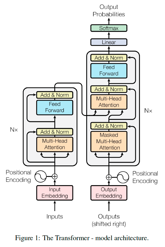
Most competitive neural sequence transduction models have an encoder-decoder structure. Here, the encoder maps an input sequence of symbol representations \((x_1, \dots, x_n)\) to a sequence of continuous representations \((z_1,\dots,z_n)\). Given \(\mathbf{z}\), the decoder then generates an output sequence \((y_1,\dots,y_m)\) of symbols one element at a time. At each step the model is auto-regressive, consuming the previously generated symbols as additional input when generating the next. The Transformer follows this overall architecture using stacked self-attention and point-wise, fully connected layers for both the encoder and decoder, shown in the left and right halves of Figure 1, respectively.

Encoder and Decoder Stacks

Encoder: The encoder is composed of a stack of \(N = 6\) identical layers. Each layer has two sub-layers. The first is a multi-head self-attention mechanism, and the second is a simple, positionwise fully connected feed-forward network. We employ a residual connection around each of the two sub-layers, followed by Layer Normalization. That is, the output of each sub-layer is

\[ \text{LayerNorm}(x+\text{Sublayer}(x)). \]

To facilitate these residual connections, all sub-layers in the model, as well as the embedding layers, produce outputs of dimension \(d_{\text{model}}=512\).

Decoder: The decoder is also composed of a stack of \(N = 6\) identical layers. In addition to the two sub-layers in each encoder layer, the decoder inserts a third sub-layer, which performs multi-head attention over the output of the encoder stack. We also modify the self-attention sub-layer in the decoder stack to prevent positions from attending to subsequent positions.

Tip

• The output of the encoder stack means the output of the last encoder layer!

• Encoder and decoder layer has the same num_steps, using mask to incorporate with different sentence length.

• In “encoder-decoder attention” layers, the queries come from the previous decoder layer, and the memory keys and values come from the output of the encoder. This allows every position in the decoder to attend over all positions in the input sequence.

Attention

An attention function can be described as mapping a query and a set of key-value pairs to an output, the output is computed as a weighted sum of the values, where the weight assigned to each value is computed by a compatibility function of the query with the corresponding key.

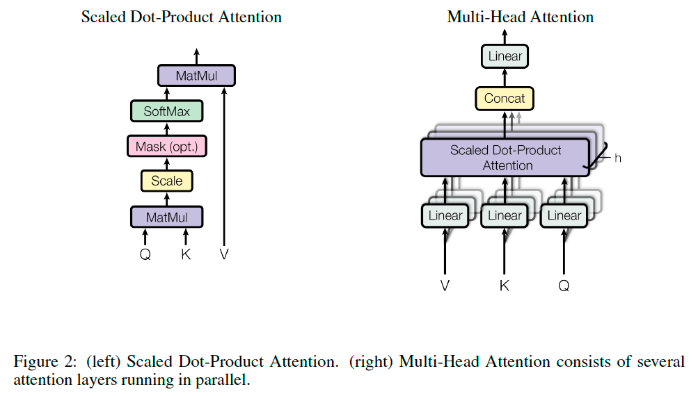
Scaled Dot-Product Attention

We call our particular attention “Scaled Dot-Product Attention” (Figure 2). The input consists of queries and keys of dimension \(d_k\), and values of dimension \(d_v\). We compute the dot products of the query with all keys, divide each by \(\sqrt{d_k}\), and apply a softmax function to obtain the weights on the values.

In practice, we compute the attention function on a set of queries simultaneously, packed together into a matrix \(Q\). The keys and values are also packed together into matrices \(K\) and \(V\). We compute the matrix of outputs as:

\[ \text{Attention}(Q, K, V) = \text{softmax}\left(\frac{QK^{T}}{\sqrt{d_{k}}}\right)V \]

Tip

We suspect that for large values of \(d_k\), the dot products grow large in magnitude, pushing the softmax function into regions where it has extremely small gradients. To counteract this effect, we scale the dot products by \(\frac{1}{\sqrt{d_k}}\).

Multi-Head Attention

We found it beneficial to linearly project the queries, keys and values \(h\) times with different, learned linear projections to \(d_k\), \(d_k\) and \(d_v\) dimensions, respectively. On each of these projected versions of queries, keys and values we then perform the attention function in parallel, yielding \(d_v\)-dimensional output values. These are concatenated and once again projected, resulting in the final values.

Multi-head attention allows the model to jointly attend to information from different representation subspaces at different positions:

\[\begin{split} \begin{aligned} \text{MultiHead}(Q, K, V) &= \text{Concat}(\text{head}_1,\dots,\text{head}_h)W^{O}\\ \text{where head}_{i} &= \text{Attention}(QW_{i}^{Q}, KW_{i}^{K}, VW_{i}^{V}) \end{aligned} \end{split}\]

Where the projections are parameter matrices \(W_{i}^{Q}\in\mathbb{R}^{d_{\text{model}}\times d_k}\), \(W_{i}^{K}\in\mathbb{R}^{d_{\text{model}}\times d_k}\), \(W_{i}^{V}\in\mathbb{R}^{d_{\text{model}}\times d_v}\) and \(W_{O}\in\mathbb{R}^{hd_{v}\times d_{\text{model}}}\).

Position-wise Feed-Forward Networks

In addition to attention sub-layers, each of the layers in our encoder and decoder contains a fully connected feed-forward network, which is applied to each position separately and identically. This consists of two linear transformations with a ReLU activation in between.

\[ \text{FFN}(x) = \max(0, xW_1+b_1)W_2 + b_2. \]

Embeddings and Softmax

Similarly to other sequence transduction models, we use learned embeddings to convert the input tokens and output tokens to vectors of dimension \(d_\text{model}\). We also use the usual learned linear transformation and softmax function to convert the decoder output to predicted next-token probabilities. In our model, we share the same weight matrix between the two embedding layers and the pre-softmax linear transformation. In the embedding layers, we multiply those weights by \(\sqrt{d_{\text{model}}}\).

Tip

The weights in word embeddings get initialized with zero mean and unit variance. The reason we increase the embedding values before the addition is to make the positional encoding relatively smaller.

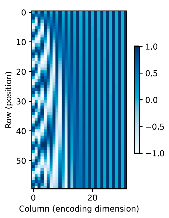
Positional Encoding

Since our model contains no recurrence and no convolution, in order for the model to make use of the order of the sequence, we must inject some information about the relative or absolute position of the tokens in the sequence. To this end, we add “positional encodings” to the input embeddings at the bottoms of the encoder and decoder stacks.

In this work, we use sine and cosine functions of different frequencies:

\[\begin{split} \begin{aligned} PE_{(pos,2i)} &= sin(pos/10000^{2i/d_{\text{model}}})\\ PE_{(pos,2i+1)} &= cos(pos/10000^{2i/d_{\text{model}}}) \end{aligned} \end{split}\]

where \(pos\) is the position and \(i\) is the dimension. That is, each dimension of the positional encoding corresponds to a sinusoid. The wavelengths form a geometric progression from \(2\pi\) to \(10000\cdot 2\pi\). We chose this function because we hypothesized it would allow the model to easily learn to attend by relative positions, since for any fixed offset \(k\), \(PE_{pos+k}\) can be represented as a linear function of \(PE_{pos}\).