TRPO

Note

TRPO updates policies by taking the largest step possible to improve performance, while satisfying a special constraint on how close the new and old policies are allowed to be.

Preliminaries

Consider an infinite-horizon discounted Markov decision process (MDP), defined by the tuple \((\mathcal{S}, \mathcal{A}, P, r, \rho_{0},\gamma)\) where \(\mathcal{S}\) is a finite set of states, \(\mathcal{A}\) is a finite set of actions, \(P: \mathcal{S}\times\mathcal{A}\times\mathcal{S}\to\mathbb{R}\) is the transition probability distribution, \(r:\mathcal{S}\to\mathbb{R}\) is the reward function (difference from our previous setting), \(\rho_{0}:\mathcal{S}\to\mathbb{R}\) is the distribution of the initial state \(s_{0}\), \(\gamma\in(0, 1)\) is the discount factor.

Let \(\pi\) denote a stochastic policy \(\pi:\mathcal{S}\times\mathcal{A}\to[0, 1]\), and let \(\eta(\pi)\) denote its expected discounted reward:

\[\eta(\pi) = \mathbb{E}_{s_0,a_0,\dots}\left[\sum_{t=0}^{\infty}\gamma^{t}r(s_{t})\right]\]

where \(s_0\sim\rho_0(s_0)\), \(a_t\sim\pi(a_t|s_t)\), \(s_{t+1}\sim P(s_{t+1}|s_{t}, a_{t})\).

The following useful identity expresses the expected return of another policy \(\tilde{\pi}\) in terms of the advantage over \(\pi\):

\[\eta(\tilde{\pi}) = \eta(\pi) + \mathbb{E}_{s_0,a_0,\dots\sim\tilde{\pi}}\left[\sum_{t=0}^{\infty}\gamma^{t}A_{\pi}(s_t,a_t)\right]\]

Tip

\[\begin{split} \begin{aligned} \mathbb{E}_{\tau\sim\tilde{\pi}}\left[\sum_{t=0}^{\infty}\gamma^{t}A_{\pi}(s_t,a_t)\right] &= \mathbb{E}_{\tau\sim\tilde{\pi}}\left[\sum_{t=0}^{\infty}\gamma^{t}(r(s_t) + \gamma V_{\pi}(s_{t+1}) - V_{\pi}(s_t))\right]\\ &= \mathbb{E}_{\tau\sim\tilde{\pi}}\left[-V_{\pi}(s_0) + \sum_{t=0}^{\infty}\gamma^{t}r(s_t)\right]\\ &= -\mathbb{E}_{s_0}[V_{\pi}(s_0)] + \mathbb{E}_{\tau\sim\tilde{\pi}}\left[\sum_{t=0}^{\infty}\gamma^{t}r(s_t)\right]\\ &= -\eta(\pi) + \eta(\tilde{\pi}) \end{aligned} \end{split}\]

Let \(\rho_{\pi}\) be the discounted visitation frequencies:

\[\rho_{\pi}(s) = P(s_0=s) + \gamma P(s_1=s) + \gamma^{2}P(s_2=s) + \dots\]

We can rewrite Equation with a sum over states instead of timesteps:

\[\begin{split} \begin{aligned} \eta(\tilde{\pi}) &= \eta(\pi) + \sum_{t=0}^{\infty}\sum_{s}P(s_{t}=s|\tilde{\pi})\sum_{a}\tilde{\pi}(a|s)\gamma^{t}A_{\pi}(s, a) \\ &= \eta(\pi) + \sum_{s}\sum_{t=0}^{\infty}\gamma^{t}P(s_{t}=s|\tilde{\pi})\sum_{a}\tilde{\pi}(a|s)A_{\pi}(s, a) \\ &= \eta(\pi) + \sum_{s}\rho_{\tilde{\pi}}(s)\sum_{a}\tilde{\pi}(a|s)A_{\pi}(s, a) \end{aligned} \end{split}\]

This equation implies that any policy update \(\pi\to\tilde{\pi}\) that has a nonnegative expected advantage at every state \(s\), i.e., \(\sum_{a}\tilde{\pi}(a|s)A_{\pi}(s, a)\ge 0\), is guaranteed to increase the policy performance \(\eta\). However, the complex dependency of \(\rho_{\tilde{\pi}}(s)\) on \(\tilde{\pi}\) makes it difficult to optimize directly. Instead, we introduce the following local approximation to \(\eta\):

\[L_{\pi}(\tilde{\pi}) = \eta(\pi) + \sum_{s}\rho_{\pi}(s)\sum_{a}\tilde{\pi}(a|s)A_{\pi}(s, a)\]

Note that \(L_{\pi}\) uses the visitation frequency \(\rho_{\pi}\) rather than \(\rho_{\tilde{\pi}}\). If we have a parameterized policy \(\pi_{\theta}\), where \(\pi_{\theta}(a|s)\) is a differentiable function of the parameter vector \(\theta\), then \(L_{\pi}\) matches \(\eta\) to first order:

\[L_{\pi_{\theta_{0}}}(\pi_{\theta_{0}}) = \eta(\pi_{\theta_{0}})\]

\[\nabla_{\theta}L_{\pi_{\theta_0}}(\pi_{\theta_0})|_{\theta=\theta_0} = \nabla_{\theta}\eta(\pi_{\theta_{0}})|_{\theta=\theta_0}\]

It implies that a sufficiently small step that improves \(L_{\pi_{\theta_{\text{old}}}}\) will also improve \(\eta\), but does not give us any guidance on how big of a step to take.

Monotonic Improvement Guarantee

To address the above issue, the author proposed a policy updating scheme, for which they could provide explicit lower bounds on the improvement of \(\eta\). Let \(\pi_{\text{old}}\) denote the current policy, denote total variation divergence \(D_{\text{TV}}(p\|q) = \frac{1}{2}\sum_{i}|p_{i} - q_{i}|\), define a distance measure between \(\pi\) and \(\tilde{\pi}\):

\[ D_{\text{TV}}^{\max}(\pi, \tilde{\pi}) = \max_{s}D_{\text{TV}}(\pi(\cdot|s)\left|\right|\tilde{\pi}(\cdot|s)) \]

Theorem 7

Let \(\alpha=D_{\text{TV}}^{\max}(\pi_{\text{old}}, \pi_{\text{new}})\). Then the following bound holds:

\[\eta(\pi_{\text{new}})\ge L_{\pi_{\text{old}}}(\pi_{\text{new}}) - \frac{4\epsilon\gamma}{(1-\gamma)^2}\alpha^{2}\]

where \(\epsilon=\max_{s,a}|A_{\pi_{\text{old}}}(s, a)|\).

Next, we note the following relationship between the total variation divergence and the KL divergence \(D_{\text{TV}}(p\|q)^{2}\le D_{\text{KL}}(p\|q)\). Let \(D_{\text{KL}}^{\max}(\pi,\tilde{\pi}) = \max_{s}D_{\text{KL}}(\pi(\cdot|s)\|\tilde{\pi}(\cdot|s))\), the following bounds then follows directly:

\[\eta(\tilde{\pi})\ge L_{\pi}(\tilde{\pi}) - CD_{\text{KL}}^{\max}(\pi,\tilde{\pi}),\]

\[\text{ where }\ C=\frac{4\epsilon\gamma}{(1-\gamma)^2}.\]

---

Algorithm 1 describes an approximate policy iteration scheme based on the policy improvement bound above. Note that for now, we assume exact evaluation of the advantage values \(A_{\pi}\).

Initialize \(\pi_{0}\)
for \(i=0,1,2,\dots\) until convergence do
\(\quad\)Compute all advantage values \(A_{\pi_{i}}(s, a)\).
\(\quad\)Solve the constrained optimization problem
\(\quad \pi_{i+1} = \arg\max_{\pi}\left[L_{\pi_{i}}(\pi) - CD_{\text{KL}}^{\max}(\pi_{i}, \pi)\right]\)
\(\quad\)\(\quad\)where \(C = 4\epsilon\gamma/(1-\gamma)^{2}\)
\(\quad\)\(\quad\)and \(L_{\pi_{i}}(\pi) = \eta(\pi_{i}) + \sum_{s}\rho_{\pi_{i}}(s)\sum_{a}\pi(a|s)A_{\pi_{i}}(s,a)\)
end for

---

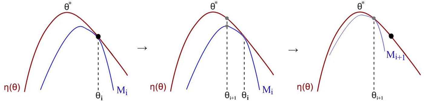
This algorithm is a type of minorization-maximization (MM) algorithm, which is guaranteed to generate a monotonically improving sequence of policies. Trust region policy optimization, which we propose in the following section, is an approximation to Algorithm 1.

Optimization of Parameterized Policies

The preceding section showed that \(\eta(\theta) \ge L_{\theta_{\text{old}}}(\theta) - CD_{\text{KL}}^{\max}(\theta_{\text{old}}, \theta)\), with equality at \(\theta_{\text{old}}=\theta\). Thus, by performing the following maximization, we are guaranteed to improve the true objective \(\eta\):

\[\underset{\theta}{\text{maximize}}\left[L_{\theta_{\text{old}}}(\theta) - CD_{\text{KL}}^{\max}(\theta_{\text{old}}, \theta)\right].\]

In practice, if we used the penalty coefficient \(C\) recommended by the theory above, the step sizes would be very small. One way to take larger steps in a robust way is to use a constraint on the KL divergence between the new policy and the old policy, i.e., a trust region constraint:

\[\underset{\theta}{\text{maximize}}L_{\theta_{\text{old}}}(\theta)\]

\[\text{subject to }D_{\text{KL}}^{\max}(\theta_{\text{old}}, \theta)\le\delta.\]

This problem imposes a constraint that the KL divergence is bounded at every point in the state space. While it is motivated by the theory, this problem is impractical to solve due to the large number of constraints. Instead, we can use a heuristic approximation which considers the average KL divergence:

\[\bar{D}_{\text{KL}}^{\rho}(\theta_1, \theta_2) :=\mathbb{E}_{s\sim\rho}\left[D_{\text{KL}}(\pi_{\theta_1}(\cdot|s)\left|\right|\pi_{\theta_2}(\cdot|s))\right]\]

We seek to solve the following optimization problem, obtained by expanding \(L_{\theta_{\text{old}}}\):

\[\underset{\theta}{\text{maximize}}\sum_{s}\rho_{\theta_{\text{old}}}(s)\sum_{a}\pi_{\theta}(a|s)A_{\pi_{\theta_{\text{old}}}}(s,a)\]

\[\text{s.t.}\ \bar{D}_{\text{KL}}^{\rho_{\theta_{\text{old}}}}(\theta_{\text{old}}, \theta)\le\delta.\]

We replace the sum over the actions by an importance sampling estimator. Using \(q\) to denote the sampling distribution:

\[\sum_{a}\pi_{\theta}(a|s)A_{\pi_{\theta_{\text{old}}}}(s,a) = \mathbb{E}_{a\sim q}\left[\frac{\pi_{\theta}(a|s)}{q(a|s)}A_{\theta_{\text{old}}}(s,a)\right]\]

Let \(q=\pi_{\theta_{\text{old}}}\), the theoretical TRPO update is:

\[\underset{\theta}{\text{maximize}}\ \mathbb{E}_{s,a\sim\pi_{\theta_{\text{old}}}}\left[\frac{\pi_{\theta}(a|s)}{\pi_{\theta_{\text{old}}}(a|s)}A_{\theta_{\text{old}}}(s,a)\right]\]

\[\text{s.t.}\ \mathbb{E}_{s\sim\pi_{\theta_{\text{old}}}}\left[D_{\text{KL}}(\pi_{\theta_{\text{old}}}(\cdot|s)\left|\right|\pi_{\theta}(\cdot|s))\right] \le \delta.\]

which is equivalent to:

\[\begin{split} \begin{aligned} \theta_{k+1} &= \arg\underset{\theta}{\max}\mathcal{L}(\theta_{k},\theta) \\ &= \arg\underset{\theta}{\max}\underset{s,a\sim\pi_{\theta_{k}}}{\mathbb{E}}\left[\frac{\pi_{\theta}(a|s)}{\pi_{\theta_{k}}(a|s)}A_{\theta_{k}}(s,a)\right]\\ \end{aligned} \end{split}\]

\[ \text{s.t.}\ \bar{D}_{KL}(\theta\left|\right|\theta_{k}) = \mathbb{E}_{s\sim\pi_{\theta_{k}}}\left[D_{\text{KL}}(\pi_{\theta}(\cdot|s)\left|\right|\pi_{\theta_{k}}(\cdot|s))\right] \le \delta.\ \]

Tip

The objective and constraint are both zero when \(\theta = \theta_k\). Furthermore, the gradient of the constraint with respect to \(\theta\) is zero when \(\theta = \theta_k\).

Approximation

The theoretical TRPO update isn’t the easiest to work with, so TRPO makes some approximations to get an answer quickly. We Taylor expand the objective and constraint to leading order around \(\theta_k\):

\[\begin{split} \begin{aligned} \mathcal{L}(\theta_{k},\theta) &\approx g^{\intercal}(\theta-\theta_{k})\\ \bar{D}_{KL}(\theta\left|\right|\theta_{k}) &\approx \frac{1}{2}(\theta-\theta_{k})^{\intercal}H(\theta-\theta_{k}) \end{aligned} \end{split}\]

resulting in an approximate optimization problem,

\[ \theta_{k+1} = \arg\underset{\theta}{\max}g^{\intercal}(\theta-\theta_{k}) \]

\[ \text{s.t.}\ \frac{1}{2}(\theta-\theta_{k})^{\intercal}H(\theta-\theta_{k}) \le\delta. \]

This approximate problem can be analytically solved by the methods of Lagrangian duality:

\[ \theta_{k+1} = \theta_k + \sqrt{\frac{2 \delta}{g^T H^{-1} g}} H^{-1} g. \]

Due to the approximation errors introduced by the Taylor expansion, the analytic solution may not satisfy the KL constraint, or actually improve the surrogate advantage. TRPO adds a modification to this update rule: a backtracking line search,

\[ \theta_{k+1} = \theta_k + \alpha^j \sqrt{\frac{2 \delta}{g^T H^{-1} g}} H^{-1} g, \]

where \(\alpha \in (0,1)\) is the backtracking coefficient, and \(j\) is the smallest nonnegative integer such that \(\pi_{\theta_{k+1}}\) satisfies the KL constraint and produces a positive surrogate advantage.

Tip

Computing and storing the matrix inverse, \(H^{-1}\), is painfully expensive when dealing with neural network policies with thousands or millions of parameters. TRPO sidesteps the issue by using the conjugate gradient algorithm to solve \(Hx = g\) for \(x = H^{-1} g\), requiring only a function which can compute the matrix-vector product \(Hx\) instead of computing and storing the whole matrix \(H\) directly. This is not too hard to do: we set up a symbolic operation to calculate

\[ Hx = \nabla_{\theta} \left( \left(\nabla_{\theta} \bar{D}_{KL}(\theta || \theta_k)\right)^T x \right), \]

which gives us the correct output without computing the whole matrix.