
Deep Q-Learning with Pytorch#
Note
This section we will show how to use PyTorch to train a Deep Q-Learning (DQN) agent on the CartPole-v1 task from Gymnasium.
Task#
The agent has to decide between two actions - moving the cart left or right - so that the pole attached to it stays upright.
As the agent observes the current state of the environment and chooses an action, the environment transitions to a new state, and also returns a reward that indicates the consequences of the action. In this task, rewards are +1 for every incremental timestep and the environment terminates if the pole falls over too far or the cart moves more than 2.4 units away from center.
Packages#
We need gymnasium for the environment, installed by using pip.
pip install gymnasium
import math
import random
import matplotlib
import matplotlib.pyplot as plt
from collections import namedtuple, deque
from itertools import count

import gymnasium as gym
import torch
import torch.nn as nn
import torch.optim as optim
import torch.nn.functional as F

env = gym.make("CartPole-v1")

# set up matplotlib
is_ipython = 'inline' in matplotlib.get_backend()
if is_ipython:
    from IPython import display

plt.ion()

# if GPU is to be used
device = torch.device("cuda" if torch.cuda.is_available() else "cpu")
Replay Memory#
We’re going to need two classes:
Transition- a named tuple representing a single transition in our environment. It essentially maps (state, action) pairs to their (next_state, reward) result, with the state being the screen difference image as described later on.ReplayMemory- a cyclic buffer of bounded size that holds the transitions observed recently. It also implements a.sample()method for selecting a random batch of transitions for training.
Transition = namedtuple('Transition',
                        ('state', 'action', 'next_state', 'reward'))


class ReplayMemory(object):

    def __init__(self, capacity):
        self.memory = deque([], maxlen=capacity)

    def push(self, *args):
        """Save a transition"""
        self.memory.append(Transition(*args))

    def sample(self, batch_size):
        return random.sample(self.memory, batch_size)

    def __len__(self):
        return len(self.memory)
Q-network#
Our model will be a feed forward neural network that takes in the difference between the current and previous screen patches. It has two outputs, representing \(Q(s, \text{left})\) and \(Q(s, \text{right})\) (where \(s\) is the input to the network).
class DQN(nn.Module):

    def __init__(self, n_observations, n_actions):
        super(DQN, self).__init__()
        self.layer1 = nn.Linear(n_observations, 128)
        self.layer2 = nn.Linear(128, 128)
        self.layer3 = nn.Linear(128, n_actions)

    # Called with either one element to determine next action, or a batch
    # during optimization. Returns tensor([[left0exp,right0exp]...]).
    def forward(self, x):
        x = F.relu(self.layer1(x))
        x = F.relu(self.layer2(x))
        return self.layer3(x)
Hyperparameters and utilities#
# BATCH_SIZE is the number of transitions sampled from the replay buffer
# GAMMA is the discount factor as mentioned in the previous section
# EPS_START is the starting value of epsilon
# EPS_END is the final value of epsilon
# EPS_DECAY controls the rate of exponential decay of epsilon, higher means a slower decay
# TAU is the update rate of the target network
# LR is the learning rate of the ``AdamW`` optimizer
BATCH_SIZE = 128
GAMMA = 0.99
EPS_START = 0.9
EPS_END = 0.05
EPS_DECAY = 1000
TAU = 0.005
LR = 1e-4
# Get number of actions from gym action space
n_actions = env.action_space.n
# Get the number of state observations
state, info = env.reset()
n_observations = len(state)

policy_net = DQN(n_observations, n_actions).to(device)
target_net = DQN(n_observations, n_actions).to(device)
target_net.load_state_dict(policy_net.state_dict())

optimizer = optim.AdamW(policy_net.parameters(), lr=LR, amsgrad=True)
memory = ReplayMemory(10000)
steps_done = 0


def select_action(state):
    global steps_done
    sample = random.random()
    eps_threshold = EPS_END + (EPS_START - EPS_END) * \
        math.exp(-1. * steps_done / EPS_DECAY)
    steps_done += 1
    if sample > eps_threshold:
        with torch.no_grad():
            # t.max(1) will return the largest column value of each row.
            # second column on max result is index of where max element was
            # found, so we pick action with the larger expected reward.
            return policy_net(state).max(1).indices.view(1, 1)
    else:
        return torch.tensor([[env.action_space.sample()]], device=device, dtype=torch.long)
episode_durations = []
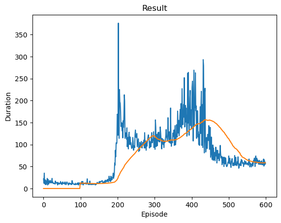
def plot_durations(show_result=False):
plt.figure(1)
durations_t = torch.tensor(episode_durations, dtype=torch.float)
if show_result:
plt.title('Result')
else:
plt.clf()
plt.title('Training...')
plt.xlabel('Episode')
plt.ylabel('Duration')
plt.plot(durations_t.numpy())
# Take 100 episode averages and plot them too
if len(durations_t) >= 100:
means = durations_t.unfold(0, 100, 1).mean(1).view(-1)
means = torch.cat((torch.zeros(99), means))
plt.plot(means.numpy())
plt.pause(0.001) # pause a bit so that plots are updated
if is_ipython:
if not show_result:
display.display(plt.gcf())
display.clear_output(wait=True)
else:
display.display(plt.gcf())
Training one step#
Here, you can find an optimize_model function that performs a single step of the optimization. It first samples a batch, concatenates all the tensors into a single one, computes \(Q(s_{t}, a_{t})\) and \(V(s_{t+1}) = \max_{a}Q(s_{t+1}, a)\), and combines them into our loss. By definition we set \(V(s)=0\) if \(s\) is a terminal state. We also use a target network to compute \(V(s_{t+1})\) for added stability. The target network is updated at every step with a soft update controlled by the hyperparameter TAU, which was previously defined.
We will use the Huber loss. The Huber loss acts like the mean squared error when the error is small, but like the mean absolute error when the error is large - this makes it more robust to outliers when the estimates of \(Q\) are very noisy.
def optimize_model():
    if len(memory) < BATCH_SIZE:
        return
    transitions = memory.sample(BATCH_SIZE)
    # Converts batch-array of Transitions to Transition of batch-arrays.
    batch = Transition(*zip(*transitions))

    # Compute a mask of non-final states and concatenate the batch elements
    # (a final state would've been the one after which simulation ended)
    non_final_mask = torch.tensor(tuple(map(lambda s: s is not None,
                                          batch.next_state)), device=device, dtype=torch.bool)
    non_final_next_states = torch.cat([s for s in batch.next_state
                                                if s is not None])
    state_batch = torch.cat(batch.state)
    action_batch = torch.cat(batch.action)
    reward_batch = torch.cat(batch.reward)

    # Compute Q(s_t, a) - the model computes Q(s_t), then we select the
    # columns of actions taken. These are the actions which would've been taken
    # for each batch state according to policy_net
    state_action_values = policy_net(state_batch).gather(1, action_batch)

    # Compute V(s_{t+1}) for all next states.
    # Expected values of actions for non_final_next_states are computed based
    # on the "older" target_net; selecting their best reward with max(1).values
    # This is merged based on the mask, such that we'll have either the expected
    # state value or 0 in case the state was final.
    next_state_values = torch.zeros(BATCH_SIZE, device=device)
    with torch.no_grad():
        next_state_values[non_final_mask] = target_net(non_final_next_states).max(1).values
    # Compute the expected Q values
    expected_state_action_values = (next_state_values * GAMMA) + reward_batch

    # Compute Huber loss
    criterion = nn.SmoothL1Loss()
    loss = criterion(state_action_values, expected_state_action_values.unsqueeze(1))

    # Optimize the model
    optimizer.zero_grad()
    loss.backward()
    # In-place gradient clipping
    torch.nn.utils.clip_grad_value_(policy_net.parameters(), 100)
    optimizer.step()
Training loop#
Below, you can find the main training loop. At the beginning we reset the environment and obtain the initial state Tensor. Then, we sample an action, execute it, observe the next state and the reward (always 1), and optimize our model once. When the episode ends (our model fails), we restart the loop.
num_episodes = 600

for i_episode in range(num_episodes):
    # Initialize the environment and get it's state
    state, info = env.reset()
    state = torch.tensor(state, dtype=torch.float32, device=device).unsqueeze(0)
    for t in count():
        action = select_action(state)
        observation, reward, terminated, truncated, _ = env.step(action.item())
        reward = torch.tensor([reward], device=device)
        done = terminated or truncated

        if terminated:
            next_state = None
        else:
            next_state = torch.tensor(observation, dtype=torch.float32, device=device).unsqueeze(0)

        # Store the transition in memory
        memory.push(state, action, next_state, reward)

        # Move to the next state
        state = next_state

        # Perform one step of the optimization (on the policy network)
        optimize_model()

        # Soft update of the target network's weights
        # θ′ ← τ θ + (1 −τ )θ′
        target_net_state_dict = target_net.state_dict()
        policy_net_state_dict = policy_net.state_dict()
        for key in policy_net_state_dict:
            target_net_state_dict[key] = policy_net_state_dict[key]*TAU + target_net_state_dict[key]*(1-TAU)
        target_net.load_state_dict(target_net_state_dict)

        if done:
            episode_durations.append(t + 1)
            plot_durations()
            break

print('Complete')
plot_durations(show_result=True)
plt.ioff()
plt.show()
Complete
<Figure size 640x480 with 0 Axes>
<Figure size 640x480 with 0 Axes>