
Gaussian Mixture Model#
Note
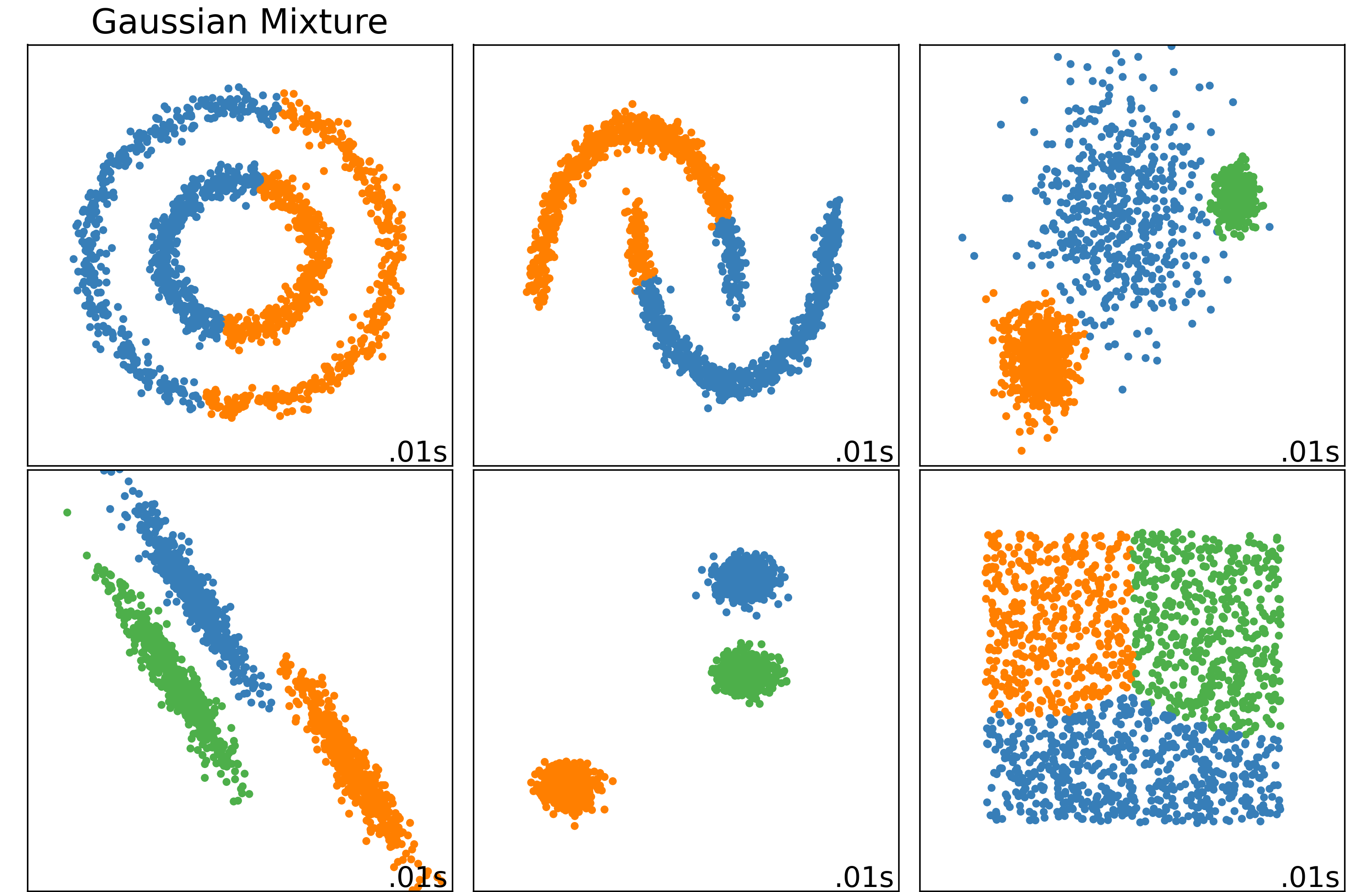
GMM assumes instances were generated from a mixture of several Gaussian distributions.
GMM uses the EM algorithm, E-step estimates which Gaussian, M-step maximizes parameters.
We can use BIC and AIC to select the number of distributions.
The simplest GMM variant which implemented in GaussianMixture must know in advance the number of Gaussian distributions \(k\).
GMM assumes instances are generated by two steps:
Estimate#
The parameters of our model are \(\phi\), \(\mu\) and \(\Sigma\). To estimate them, we can write down the likelihood of our data:
No closed form solution to this MLE problem, while if we knew what \(z^{(i)}\)’s were, the problem would have been easy.
The EM algorithm iteratively estimates \(z^{(i)}\) and maximizes parameters:
the E-step tries to estimate \(z^{(i)}\), more precisely:
the M-step maximizes the parameters of based on our guesses:
Examples#
import numpy as np
from sklearn.mixture import GaussianMixture

X = np.array([[1, 2], [1, 4], [1, 0], [10, 2], [10, 4], [10, 0]])
# need to assign n_components
gm = GaussianMixture(n_components=2, random_state=0).fit(X)
# phi
gm.weights_
array([0.5, 0.5])
# mu
gm.means_
array([[10.,  2.],
       [ 1.,  2.]])
# Sigma
gm.covariances_
array([[[1.00000000e-06, 1.15699599e-29],
        [1.15699599e-29, 2.66666767e+00]],

       [[1.00000000e-06, 1.24902977e-30],
        [1.24902977e-30, 2.66666767e+00]]])
predict#
X_predict = np.array([[0, 1], [11, 5]])
gm.predict(X_predict)
array([1, 0])
gm.predict_proba(X_predict)
array([[0., 1.],
       [1., 0.]])
sample#
# as a generative model, we can sample new instances from it
X_new, y_new = gm.sample(7)
X_new, y_new
(array([[ 9.99844709,  3.21101447],
        [ 9.99866645, -1.70416514],
        [ 9.99803008,  0.62383712],
        [ 1.00050588,  4.06756329],
        [ 0.99891919,  6.15629625],
        [ 0.99942086,  2.79087858],
        [ 0.9985898 ,  1.70347684]]),
 array([0, 0, 0, 1, 1, 1, 1]))
# log of probability density function(PDF)
gm.score_samples(X_new)
array([2.40556655, 0.42448816, 1.59092314, 2.95683262, 0.06321552,
       3.60133524, 2.87549155])
Selecting the Number of Distributions#
GMM use metrics such as Bayesian information criterion (BIC) or the Akaike information criterion (AIC):
where \(n\) is the number of instances, \(p\) is the number of parameters, \(\hat{L}\) is the likelihood.
Both BIC and AIC penalize models that have more parameters to learn and reward models that fit the data well.
"""
select k that minimize bic or the elbow of bic.
"""
gm.bic(X)
-20.92644270457478
gm.aic(X)
-18.635796866083382