Linear Regression Variants

Note

Linear Regression + L2 regularization = Ridge
Linear Regression + L1 regularization = Lasso
Linear Regression + PolynomialFeatures = Polynomial Regression

Ridge

To lower variance \(\Rightarrow \) limit model’s complexity \(\Rightarrow \) prevent the absolute value of parameters to be large \(\Rightarrow \) we add punishment term concerning the absolute value of parameters on \(J(\theta)\).

Ridge is linear regression plus the \(l_{2}\) regularization term:

\[\underset{w}{\min}\left \|Xw - y \right \|_{2}^{2} + \alpha\left \|w \right \|_{2}^{2}\]

where \(\alpha\) is the regularization hyperparameter.

import numpy as np

n_samples, n_features = 10, 5
rng = np.random.RandomState(0)
X = rng.randn(n_samples, n_features)
y = rng.randn(n_samples) 

from sklearn.linear_model import Ridge

clf = Ridge(alpha=1.0)
clf.fit(X, y)

Ridge()

Lasso

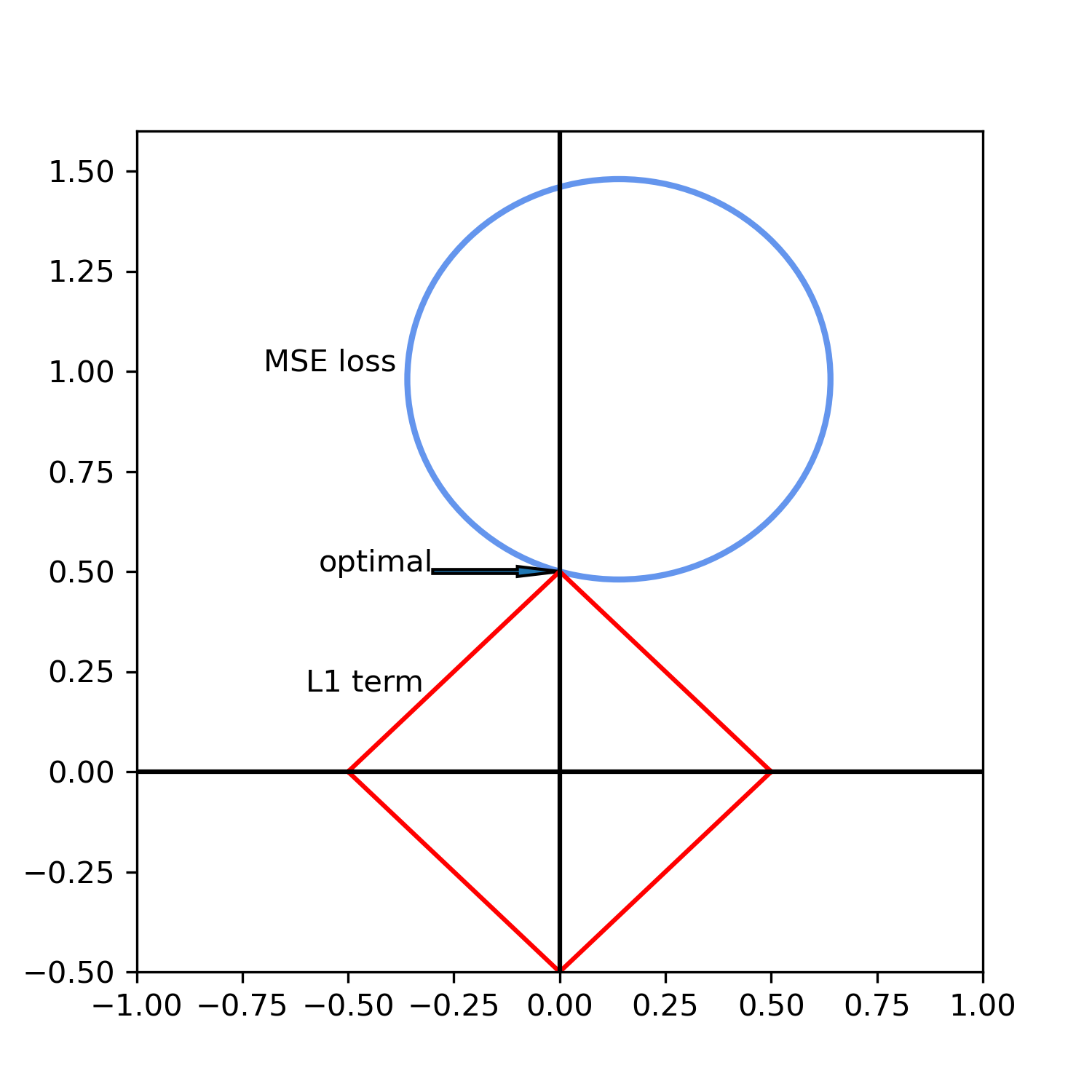
Lasso(Least Absolute Shrinkage and Selection Operator) is linear regression plus the \(l_{1}\) regularization term:

\[\underset{w}{\min}\frac{1}{2n_{samples}}\left \|Xw - y \right \|_{2}^{2} + \alpha\left \|w \right \|_{1}\]

Lasso can result in sparse parameters:

from sklearn import linear_model

reg = linear_model.Lasso(alpha=0.1)
reg.fit([[0, 0], [1, 1]], [0, 1])

reg.predict([[1, 1]])

array([0.8])

Polynomial Regression

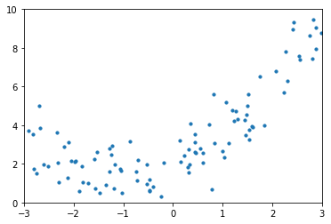
"""manual dataset"""
import matplotlib.pyplot as plt
import numpy as np

m = 100
X = 6 * np.random.rand(m, 1) - 3
y = 0.5 * X ** 2 + X + 2 + np.random.randn(m, 1)

plt.scatter(X, y, s=10)
plt.axis([-3, 3, 0, 10])
plt.show()

"""
polynomial regression = PolynomialFeatures + LinearRegression
"""
from sklearn.preprocessing import PolynomialFeatures
from sklearn.linear_model import LinearRegression

poly_features = PolynomialFeatures(degree=2, include_bias=False)
X_poly = poly_features.fit_transform(X)

lin_reg = LinearRegression()
lin_reg.fit(X_poly, y)

LinearRegression()

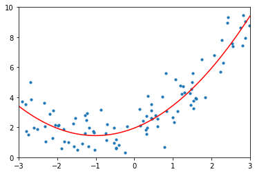
X_new=np.linspace(-3, 3, 100).reshape(100, 1)
X_new_poly = poly_features.transform(X_new)
y_new = lin_reg.predict(X_new_poly)

plt.scatter(X, y, s=10)
plt.plot(X_new, y_new, c='r')
plt.axis([-3, 3, 0, 10])
plt.show()