Linear SVM

Note

The intuition behind Support Vector Machine(SVM) is to separate positive&negative samples by large margins.

Margin

Suppose we have a binary classification problem with \(x \in \mathbb{R}^{d}, y \in \{-1, 1\}\). Try to solve this by linear classifier \(h(x) = w^{T}x + b\), if \(h(x) >= 0\) predict 1, else -1. Intuitively, in addition to correctly separate the data, we want to separate the data by large margins.

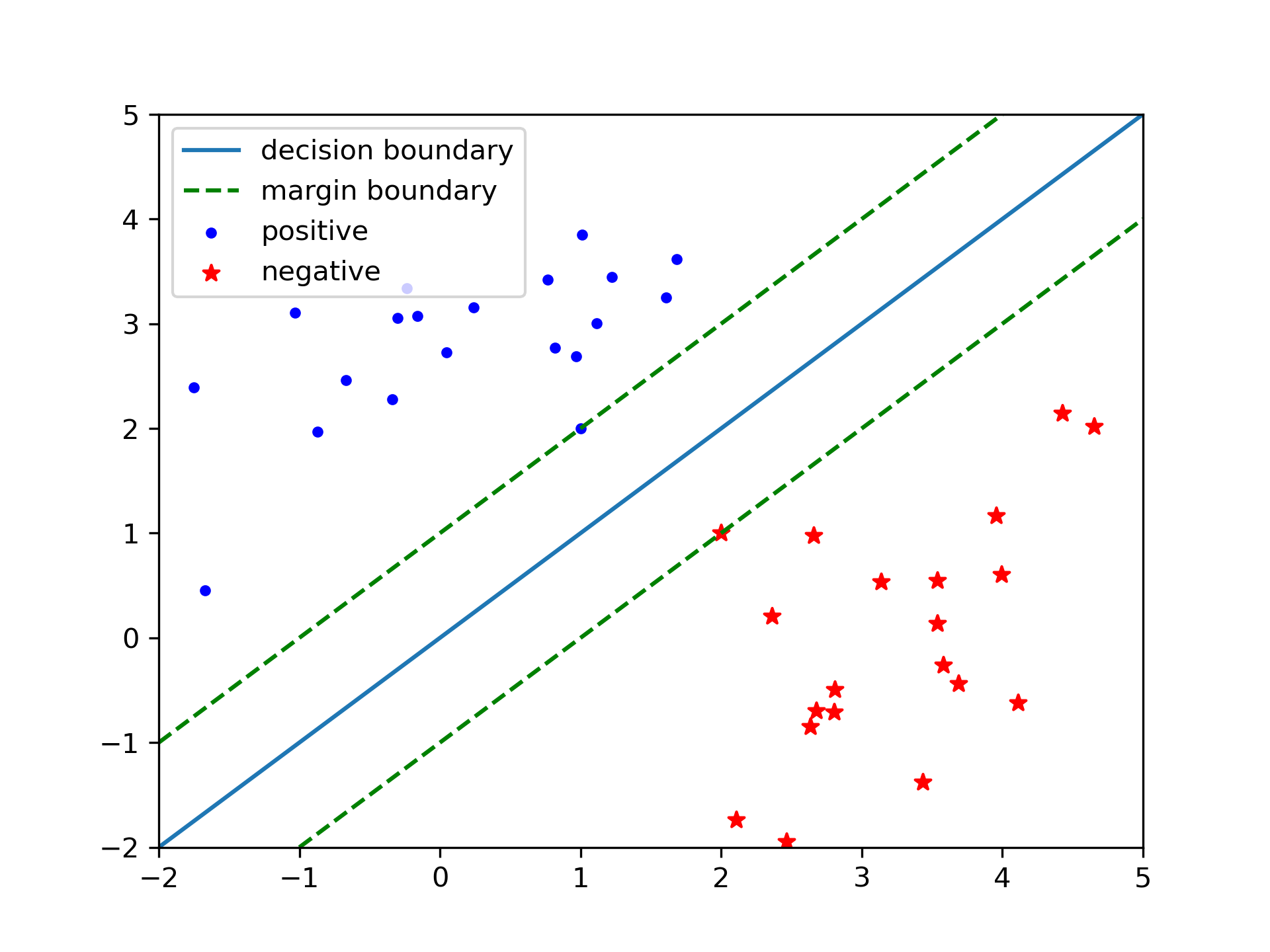
Geometric margin of the classifier:

\[\gamma^{(i)}=\frac{y^{(i)}(w^{T}x^{(i)} + b)}{\left \| w \right \| }\]

We want to maximize geometic margin:

\[\begin{split} \begin{equation} \begin{split} \underset{\gamma, w, b}{\max}\ &\gamma \\ \mbox{s.t.}\ &\frac{y^{(i)}(w^{T}x^{(i)} + b)}{\left \| w \right \| } >= \gamma \end{split} \end{equation} \end{split}\]

Without loss of generality, set \(\gamma\left \| w \right \|=1\), then the above is equivalent to:

\[\begin{split} \begin{equation} \begin{split} \underset{w, b}{\min}\ &\frac{1}{2}{\left \| w \right \|}^2 \\ \mbox{s.t.}\ &{y^{(i)}(w^{T}x^{(i)} + b)} >= 1 \end{split} \end{equation} \end{split}\]

Dual Problem

We can write the constraints as:

\[g_{i}(w) = 1 - y^{(i)}(w^{T}x^{(i)} + b) \le 0\]

The generalized Lagrangian of the above optimal problem:

\[ L(w,b,\alpha )=\frac{1}{2}\left \| w \right \|^{2} + \sum_{i=1}^{n}\alpha_{i}\left [ 1 - y^{(i)}(w^{T}x^{(i)} + b) \right ] \]

Primal problem:

\[\underset{w, b}{\min}\ \underset{\alpha_{i}\ge0}{\max}\ L(w, b, \alpha)\]

The KKT condition:

1. \(\frac{1}{2}\left \| w \right \|^{2}\) is convex.

2. \(g_{i}\)’s are convex.

3. the constraints \(g_{i}\)’s are strictly feasible.

is satisfied in the separable case, so the primal problem is equivalent to the dual problem:

\[\underset{\alpha_{i}\ge0}{\max}\ \underset{w, b}{\min}\ L(w, b, \alpha)\]

Minimize \(\nabla_{w}L(w, b, \alpha)\):

\[\nabla_{w}L(w, b, \alpha) = w - \sum_{i=1}^{n}\alpha_{i}y^{(i)}x^{(i)} = 0 \Rightarrow w = \sum_{i=1}^{n}\alpha_{i}y^{(i)}x^{(i)}\]

\[\nabla_{b}L(w, b, \alpha) = \sum_{i=1}^{n}\alpha_{i}y^{(i)}=0\]

Plug back to Lagrangian:

\[\begin{split} \begin{equation} \begin{split} L(w, b, \alpha) =& \frac{1}{2}\left \| w \right \|^{2} + \sum_{i=1}^{n}\alpha_{i}\left [ 1 - y^{(i)}(w^{T}x^{(i)} + b)\right ]\\ =& \sum_{i=1}^{n}\alpha_{i} - \sum_{i,j=1}^{n}y^{(i)}y^{(j)}\alpha_{i}\alpha_{j}(x^{(i)})^{T}x^{(i)} \end{split} \end{equation} \end{split}\]

Dual problem:

\[\begin{split} \begin{equation} \begin{split} \underset{\alpha}{\max}\ &\sum_{i=1}^{n}\alpha_{i} - \sum_{i,j=1}^{n}y^{(i)}y^{(j)}\alpha_{i}\alpha_{j}\left \langle x^{(i)},x^{(j)} \right \rangle \\ \mbox{s.t.}\ &\alpha_{i}\ge{0}, i=1,...,n \\ &\sum_{i=1}^{n}\alpha_{i}y^{(i)}=0 \end{split} \end{equation} \end{split}\]

Non-separable Case

For non-separable case, we add the soft term \(\xi\), thus transform the optimization:

\[\begin{split} \begin{equation} \begin{split} \underset{w, b}{\min}\ &\frac{1}{2}{\left \| w \right \|}^2 + C\sum_{i=1}^{n}\xi_{i}\\ \mbox{s.t.}\ &{y^{(i)}(w^{T}x^{(i)} + b)} >= 1 - \xi_{i},\ i=1,...,n\\ &\xi_{i} \ge 0,\ i=1,...,n. \end{split} \end{equation} \end{split}\]

Lagrangian:

\[ L(w,b,\xi,\alpha,r )=\frac{1}{2}\left \| w \right \|^{2} + C\sum_{i=1}^{n}\xi_{i} + \sum_{i=1}^{n}\alpha_{i}\left [1 - \xi -y^{(i)}(w^{T}x^{(i)} + b)\right ] -\sum_{i=1}^{n}r_{i}\xi_{i} \]

Dual problem of the non-separable case:

\[\begin{split} \begin{equation} \begin{split} \underset{\alpha}{\max}\ &\sum_{i=1}^{n}\alpha_{i} - \sum_{i,j=1}^{n}y^{(i)}y^{(j)}\alpha_{i}\alpha_{j}\left \langle x^{(i)},x^{(j)} \right \rangle \\ \mbox{s.t.}\ &0 \le \alpha_{i}\le{C},\ i=1,...,n \\ &\sum_{i=1}^{n}\alpha_{i}y^{(i)}=0 \end{split} \end{equation} \end{split}\]

Examples

from sklearn.datasets import make_classification

X, y = make_classification(n_features=4, random_state=0)

"""preprocessing + svm"""
from sklearn.svm import LinearSVC
from sklearn.pipeline import make_pipeline
from sklearn.preprocessing import StandardScaler

clf = make_pipeline(StandardScaler(), LinearSVC(random_state=0, tol=1e-5))
clf.fit(X, y)

Pipeline(steps=[('standardscaler', StandardScaler()),
                ('linearsvc', LinearSVC(random_state=0, tol=1e-05))])

clf.named_steps['linearsvc'].coef_

array([[0.14144316, 0.52678399, 0.67978685, 0.49307524]])

clf.predict([[0, 0, 0, 0]])

array([1])

SMO algorithm

We can not directly use coordinate ascent in SVM:

\[\begin{split} \begin{equation} \begin{split} \underset{\alpha}{\max}\ &\sum_{i=1}^{n}\alpha_{i} - \sum_{i,j=1}^{n}y^{(i)}y^{(j)}\alpha_{i}\alpha_{j}\left \langle x^{(i)},x^{(j)} \right \rangle \\ \mbox{s.t.}\ &0 \le \alpha_{i}\le{C},\ i=1,...,n \\ &\sum_{i=1}^{n}\alpha_{i}y^{(i)}=0 \end{split} \end{equation} \end{split}\]

If we want to update some \(\alpha_{i}\), we must update at least two of them simutaneously, coordinate ascent change to:

1. select some pair \(\alpha_{i}, \alpha_{j}\).

2. optimize with respect to \(\alpha_{i}, \alpha_{j}\) while holding other \(\alpha_{k}\) fixed.

We can easily change step-2 into a quatratic optimization problem.

Remaining the choice of \(\alpha_{i},\alpha_{j}\) , in fact this step is heuristic.