PCA

PCA#

Note

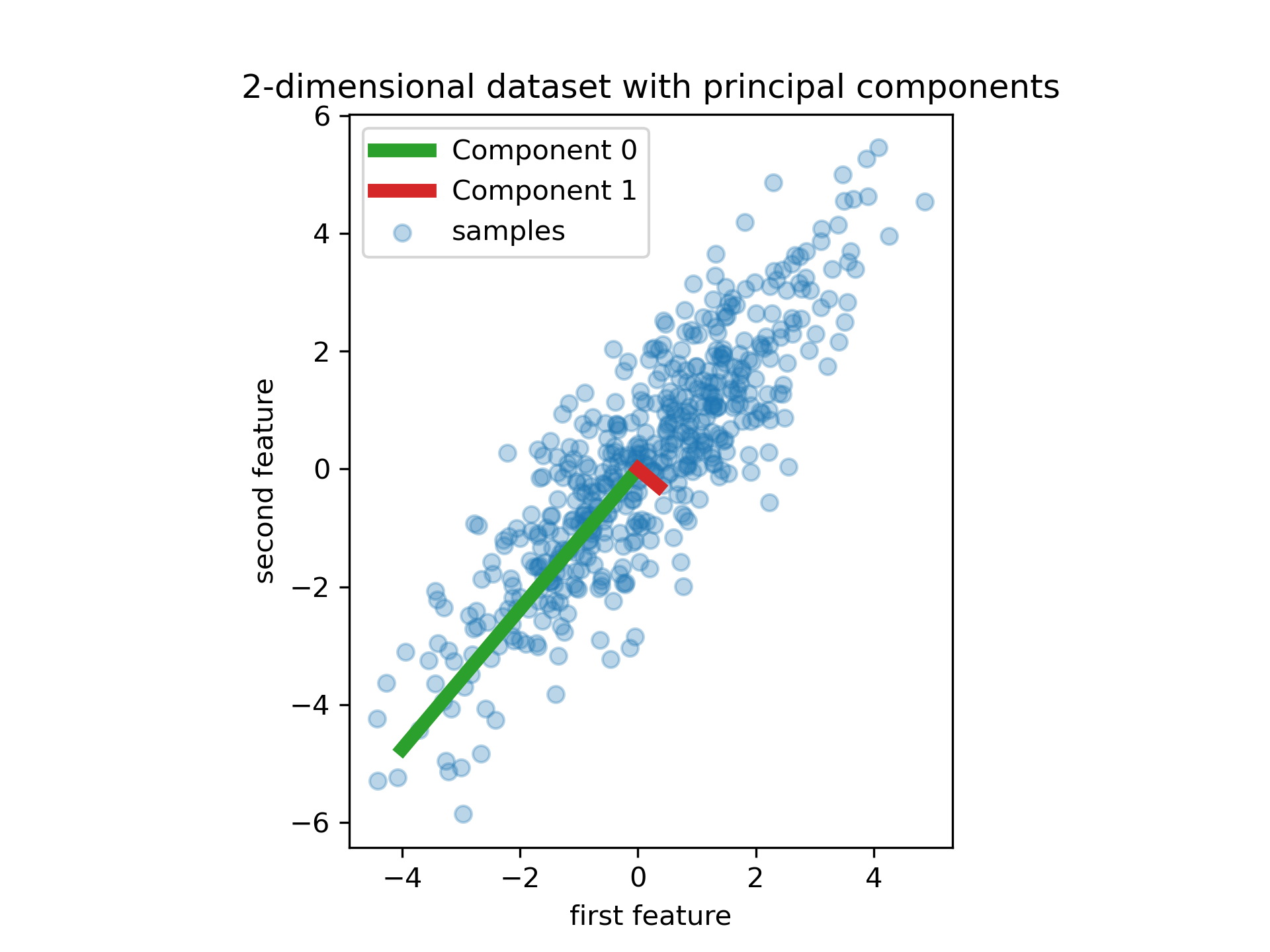
Principal Component Analysis(PCA) is by far the most popular dimentionality reduction algorithm.

First it identifies the hyperplane that lies closest to the data, then projects the data onto that hyperplane.

To choose the right hyperplane, PCA select the axis that preserve the maximum amount of variance, called the 1-th principal component.

It also finds a second axis, orthogonal to the first one, that accounts for the largest amount of remaining variance, called the 2-th principal component, and so on.

Maximize variance \(\Leftrightarrow\) Minimize the mean squared distance, because when we count translation:

\[\mbox{axis variance} + \mbox{mean square distance to axis} = \mbox{variance(which is constant)}\]

Singular Value Decomposition#

Given a \(m\times{n}\) matrix \(\mathbf{X}\), we can decompose it as:

\[\mathbf{X} = \mathbf{U}\mathbf{\Sigma}\mathbf{V}^{T}\]

where \(\mathbf{U}\), \(\mathbf{V}\) is orthogonal, \(\mathbf{\Sigma}\) is diagonal.

principal components of \(\mathbf{X}\) \(\Leftrightarrow\) columns of \(\mathbf{V}\) \(\Leftrightarrow\) eigenvectors of covariance matrix of \(\mathbf{X}\).

Examples#

"""
manual dataset
"""
import numpy as np

m = 100
w1, w2 = 0.1, 0.3
noise = 0.2

X = np.empty((m, 3))
X[:, :2] = np.random.multivariate_normal([0, 0], [[2, 1], [1, 5]], m)
# almost linear dependent
X[:, 2] = X[:, 0] * w1 + X[:, 1] * w2 + noise * np.random.randn(m)

from sklearn.decomposition import PCA

pca = PCA(n_components=2)
# fit + transform
X2D = pca.fit_transform(X)

# 1-th PCA variance ratio, 2-th PCA variance ratio, almost add up to 1
pca.explained_variance_ratio_

array([0.76240779, 0.23294253])

Choosing the Right Number of Dimensions#

"""
dimension that just preserve over 95% of variance
after training
"""
cumsum = np.cumsum(pca.explained_variance_ratio_)
d = np.argmax(cumsum >= 0.95) + 1
d

"""
set n_components to indicate the ratio of variance you wish to preserve
no need to run again
"""
pca = PCA(n_components=0.95)

Incremental PCA#

Incremental PCA split the training set into mini-batches and feed them one mini-batch at a time.

This is useful for large training sets and for applying PCA online.

from sklearn.decomposition import IncrementalPCA

n_batches = 5
inc_pca = IncrementalPCA(n_components=2)
# split X_train into 5 batches
for X_batch in np.array_split(X, n_batches):
    # partial_fit instead of fit
    inc_pca.partial_fit(X_batch)
    
X_reduced = inc_pca.transform(X)

Kernel PCA#

Using the kernel trick, KernelPCA is good at preserving clusters of instances after projection.

from sklearn.decomposition import KernelPCA

# rbf kernel is applied
rbf_pca = KernelPCA(n_components=2, kernel="rbf", gamma=0.04)
X_reduced = rbf_pca.fit_transform(X)

Tune Dimensionality Reduction#

As Dimensionality Reduction is unsupervised, there is no abvious performance measure.

While dimentionality reduction is often a preparation step for a supervised learning task.

So we can use grid search to select the hyperparameters that lead to the best performance on that task.

PCA

Contents